 Since the OneNote desktop app is getting a reprieve from its previously-announced retirement, and the anointed successor UWP app is itself being put on notice, maybe it’s worth looking at a few tweaks which can make the old app a bit more useful. There were a load of updates announced about a year ago, and further improvements to the OneNote family are on the way too.
If you use OneNote to take meeting notes – especially if you’re meeting virtually and want to have your notes alongside the Teams/Zoom/Chime app – then it makes sense to arrange the windows side by side. Students of ToW past will know that in Windows 11, pressing WindowsKey+ ← or → will snap the current window to the sides of your display, and there are other ways to control window placement if you have especially complex desktop arrangements.
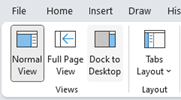
 There is an old feature in OneNote which is worth revisiting; Dock to Desktop. Invoke it at any time by pressing CTRL+ALT+D or go to the View tab to select it.
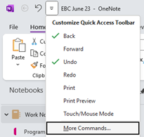
You could also try pinning it to the Quick Access Toolbar on the very top left of the OneNote window. The QAT in Office apps was covered way back in ToW #321, from March 2016.
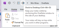 Docking has the effect of minimizing the UI for OneNote and sending it to a (horizontally resizable) section of your screen, on right-hand-side.
Usefully, it also means other apps respect that space, so even if you maximize another window, it will only grow to appear alongside your docked OneNote.
If you don’t like the position of the docked window, drag it using the “…” at the top of the pane, and position it on the top, bottom or the left side of the screen instead. If you press CTRL+ALT+D again while docked, it will fill the entire screen – maybe useful if you have a 2nd monitor.
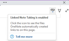
The rest of the minimal UI lets you access the pen menu, restore back to the full UI or you can use a somewhat obscure feature called Linked Notes. This will add a link back to another 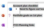 document that you could also be working on; you’ll see an icon showing the source document when you select text that has been linked.
Hover over the icon and you can get a summary or thumbnail of the document, and left-click the icon to open the document.
The original intent with Linked Notes was that you could use it across Office apps and also when browsing the web; how useful to be able to make notes on a specific web page and then jump back to the source when revisiting the notes you took! Sadly, the feature was integrated only to the dearly departed Internet Explorer, and it is not available in modern browsers. The topic of Edge support has been raised in online forums but thus far, responses have been less than forthcoming.
Even the Help page on Linked Notes talks about how it works with Word 2013, PowerPoint 2013 and other OneNote 2013 pages… no mention of Excel either.
 If you do find yourself going back in time and using Linked Notes, you’ll see an additional icon (when un-docked and back in full OneNote mode) in the top right of any page where you have links, allowing you to go straight to the source docs or to manage the links themselves.
