|
May the F4 be with you One of the neatest features in Office yet largely hidden; the F4 key repeats the last command without needing to faff about selecting the option from the menu. So what, you might say? Well, what if you’re formatting cells and want to repeat the same format over and over again – you could change one, then use the Format Painter option to apply that to select other cells, or possibly just apply the format you want, then select each additional cell in turn and press F4. One slight downside is that it only repeats the very last action, so changing a number format and then making it bold wouldn’t be easily repeatable since those are two actions. Still, there are so many uses for this “Magic Key no one knows about”. CTRL+y does the same thing in case you’ve got one of those annoying keyboards where the function keys do other things, you never know without looking if you’ll be pressing F4 or changing the system volume.
Layouts and Tabs Now, Windows has lots of tricks for arranging application windows side by side, especially if you have multiple monitors; there’s a particularly shiny new way of doing it in Windows 11 with Snap Layouts. In the context of Excel, that’s OK if you’re using two spreadsheets side by side and you might want to reference or copy data between them, but Excel has its own window-handling functions that could be more useful.
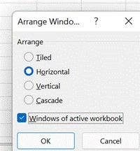
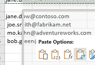
The Synchronous scrolling feature means Click on the Arrange All menu option to automatically distribute the open Excel windows, optionally confining the process to just the windows from the active workbook. Transpose data with paste It’s a fairly common exercise to take a load of data that’s in one format and want to represent it differently; there is a useful Transpose feature that takes data from columns and paste it back as a row, or vice versa. One useful scenario could be when you want to take the names of everyone who got an email or meeting request and put them in a tabular format.
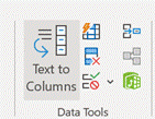
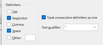
Now you have a list of addresses on their own row, and without the “;”s, but they do have a leading space ahead of all but the first one. It might be quick to correct each line in turn, and there’s always the TRIM function which could be used to tidy stuff up through formulae.
When you’re happy, remove the original line that had the text in columns, leaving just the separate email addresses on their own rows. Now, snacks just make you hungry, don’t they? |
Tag: Paste
542 –Excel Special Paste
|
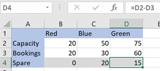
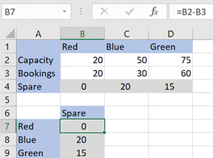
As an example, if you took the small table below and wanted to copy and paste the calculated values on row 4, you’d need to deal with the fact that the formula will change – offsetting the D and the 2 reference to wherever you paste it (eg if you pasted the copy into E4, the formula would be =E2-E3) – normally, a powerful and useful function, but a potential nuisance.
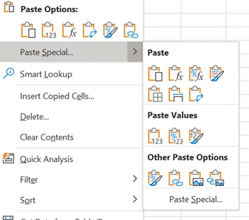
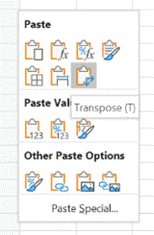
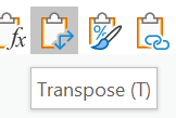
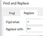
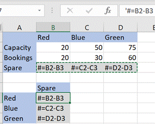
An older UI for selecting the options is available if you click on the Paste Special… command at the bottom of the pop-out, or by pressing CTRL+ALT+V to pop out the Special dialog. One of the more particularly useful features of Paste Special in Excel is the Transpose option – if you select and Copy a row of data then Paste / Transpose it, the data is rearranged as a column (and vice versa). Great news in many cases, but if you want to paste cells and keep the original formulae (without resorting to using absolute references formula references using $ in the formula itself, eg setting =$D$2-$D$3), there are no default options to transpose the orientation of the cells but not change the formulae. One trick if you ever find yourself in this position, is to bulk change the formulas so they won’t get modified when you paste the cells; do a Find & Replace to change = to something like #=. After pasting and transposing, reverse the process to restore the formula
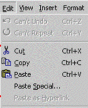
It’s an edge case but could save you lots of time if you need to do it. For most of us, getting to grips with shortcut keys in Excel would make things more productive – as well as numerous combos of CTRL-something, there are simple keys (like pressing F4, which repeats the very last command … so if you’ve just coloured a cell yellow, move the cursor to another cell and hit F4 to make that one yellow too… if you’re doing very repetitive things, this can save so much time). There are also more complex sequences; press the ALT key in Excel (and other Office apps, too) to see the key combos that A little bit of legacy/history – press ALT-E then S to jump to the Paste Special menu – why E? Even though it’s long gone, really old versions of Excel had an Edit menu, and the commands on any menu – in any application – that have an underscore under a letter (like Paste Special) are highlighting the key you can press to jump to that command. So ALT E / S used to be the combo to get Paste Special circa Excel 2003, and it still exists today. |
Tip o’ the Week 482 – Paste History
|






![clip_image002[4] clip_image002[4]](https://tipoweek.azurewebsites.net/wp-content/uploads/2019/05/clip_image0024_thumb-1.gif)
![clip_image004[4] clip_image004[4]](https://tipoweek.azurewebsites.net/wp-content/uploads/2019/05/clip_image0044_thumb.jpg)
![clip_image006[4] clip_image006[4]](https://tipoweek.azurewebsites.net/wp-content/uploads/2019/05/clip_image0064_thumb-1.gif)
![clip_image008[4] clip_image008[4]](https://tipoweek.azurewebsites.net/wp-content/uploads/2019/05/clip_image0084_thumb.gif)