|
 Anyone who has delved into writing formulæ in Excel will probably have had to manipulate strings of text at some point, possibly to clean up formatting or to convert what Excel thinks is a simple block of text into more meaningful data that we know it to be, like a number or a date. Anyone who has delved into writing formulæ in Excel will probably have had to manipulate strings of text at some point, possibly to clean up formatting or to convert what Excel thinks is a simple block of text into more meaningful data that we know it to be, like a number or a date.
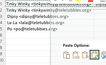
There are simple ways of bulk handling text without resorting to writing a formula – copy all the names from the To: line in an Outlook email, for example: paste into a new spreadsheet and you’ll end up with  a single line of text containing all of the display names and email addresses in one cell, which you may want to split up, to be of much use. a single line of text containing all of the display names and email addresses in one cell, which you may want to split up, to be of much use.
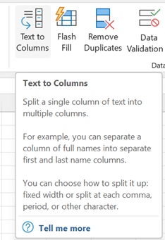
 Separate the text into multiple columns by selecting the first cell, then go to the Data tab and look for Text to Columns, which presents a fairly powerful if somewhat old-fashioned looking dialog box, to step through fixing up your text. Separate the text into multiple columns by selecting the first cell, then go to the Data tab and look for Text to Columns, which presents a fairly powerful if somewhat old-fashioned looking dialog box, to step through fixing up your text.
In the example above, we have a “;” separating – or “delimiting” – each address, so  we’ll use that to split the text across multiple columns. we’ll use that to split the text across multiple columns.
 Since we might want to create a table of names / addresses, select the cells spread across the columns, copy or cut them to the clipboard, then on a new line below, right-click and look for the Transpose option under Paste Special. Once that’s done, feel free to delete the original top row, or clear the contents of the first cell as we might come back to that row to add column names later. Since we might want to create a table of names / addresses, select the cells spread across the columns, copy or cut them to the clipboard, then on a new line below, right-click and look for the Transpose option under Paste Special. Once that’s done, feel free to delete the original top row, or clear the contents of the first cell as we might come back to that row to add column names later.
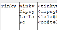
There is some other cleaning up to do with this text, though; the Text-to-Columns function chopped everything at the “;” but there’s a space which follows the semicolon, so all the Display Names after the first one have a leading space. We could repeat the Text-to-Column feature on the selection again, but use a Space as delimiter now –  unfortunately that would mangle the display names into multiple columns, and if we had a smattering of users with middle names or 3 or 4 part names common in many countries, it could make things look even worse. unfortunately that would mangle the display names into multiple columns, and if we had a smattering of users with middle names or 3 or 4 part names common in many countries, it could make things look even worse.
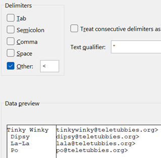
 Using the leading “<” of the email address as the delimiter is probably simplest, as it will separate the name(s) and email addresses out, though it does still give us a few tidying-up challenges, as there are spaces we don’t want and a trailing “>” at the end of every email address. Using the leading “<” of the email address as the delimiter is probably simplest, as it will separate the name(s) and email addresses out, though it does still give us a few tidying-up challenges, as there are spaces we don’t want and a trailing “>” at the end of every email address.
In cases like this, it’s easier to use a formula to clean things up – the Trim function being a good place to start; it removes both trailing and leading spaces in string, so the name can be fixed up into a new column.
Since we know the email address has one errant character – that trailing “>” – left behind from the earlier text-to-column operation, there are a variety of ways to strip it off. There’s the =LEFT() function, which keeps the left-most (n) characters of a string – so by combing the LEN function and knocking off a single character, we can chop the final character off. =LEFT() function, which keeps the left-most (n) characters of a string – so by combing the LEN function and knocking off a single character, we can chop the final character off.
After all this palaver, you might be thinking that some of this  chopping around and formulaic string-handling can get a bit confusing as you start to nest operations within each other. Luckily, the Excel team has released some powerful new text-handling functions to try to simplify things a little: chopping around and formulaic string-handling can get a bit confusing as you start to nest operations within each other. Luckily, the Excel team has released some powerful new text-handling functions to try to simplify things a little:
- TEXTBEFORE – Returns text that’s before delimiting characters
- TEXTAFTER – Returns text that’s after delimiting character
- TEXTSPLIT – Splits text into rows or columns using delimiters
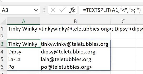
 So, using TEXTSPLIT on our original pasted text from the email, using “<” as the delimiter for the columns and “>; “ as the marker for the end of each row, gives us a near perfect solution – the only clanger being the trailing “>” on the last address. So, using TEXTSPLIT on our original pasted text from the email, using “<” as the delimiter for the columns and “>; “ as the marker for the end of each row, gives us a near perfect solution – the only clanger being the trailing “>” on the last address.
You could use another formula to find and strip out any left-over characters like that, or just manually delete the last “>” off the original line you pasted in.
You decide.
|


